In this post
People use vectors in physics mostly, and they give a relationship between two different directions. A vector can be thought of as a journey which has two different ways of being described:
- With components
- With a distance and direction
What this means is that we can describe the ‘journey’ by moving straight to the destination after being given the angle or we can move along horizontally and then vertically upwards. Since we know that the hypotenuse of a right-angled triangle squared is equal to the other sides squared and then added together, we can relate the two directions.
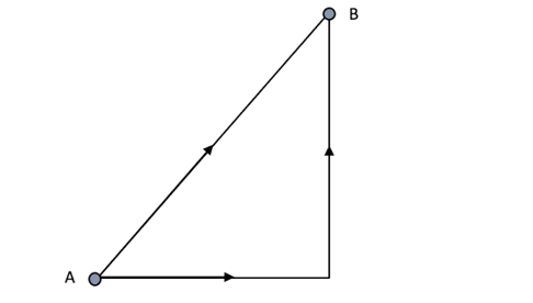
To get from A to B we can go along the hypotenuse of the triangle or go along the bottom edge and then up. Therefore, if we can relate these two we will not even need to know a direction, we would just need to know how far along and then how far up we must travel. This is where vectors are very useful!
Notation
To find out how far along and then up we must travel to end up at the same destination as going along the hypotenuse, we need to use notation. For this we use the letters and.
the distance horizontally that we must travel
the distance vertically that we must travel
So if we were to write a distance of moving 4 along and 5 up we could write this as 4i+5j. This could then be shown in a grid to find the total distance travelled:
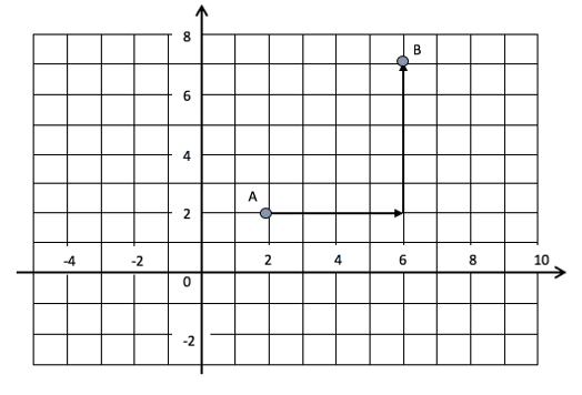
We write the vector with components i and j in bold to make sure that we do not think that they are unknowns. Sometimes you may see them with a small squiggle (~) underneath or on top of the letters i and j. This again denotes that the letter is representing a vector. The start and finishing points of the vector, say points A and B, are used to name the particular vector. So above we have:
![Rendered by QuickLaTeX.com \[ \vec{AB} \]](https://b3801007.smushcdn.com/3801007/wp-content/ql-cache/quicklatex.com-1ab07a848a78cfe6707e3090324fe778_l3.png?lossy=2&strip=1&webp=1)
or ‘vector AB’. The arrow on top of the letters simply tells us that we are working with a vector that goes from point A to point B.
When looking at vectors, a wide range of different terminology and notations can be used. Getting to know all of these can be tricky, but one of the main things to remember is that a vector can be named as being:
where A and B are two separate points. This shows that the vector is essentially the length and angle of a line that travels from point A to point B. Below we can see two different vectors that are in different locations:
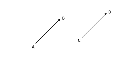
These two vectors can be labelled as:
![Rendered by QuickLaTeX.com \[ \vec{AB} \text{and} \vec{CD} \]](https://b3801007.smushcdn.com/3801007/wp-content/ql-cache/quicklatex.com-ff13a86e091969e4ad73e43eb89ec964_l3.png?lossy=2&strip=1&webp=1)
and are the same length and direction despite being in different locations. This means that we can say that:
![Rendered by QuickLaTeX.com \[ \vec{AB} = \vec{CD} \]](https://b3801007.smushcdn.com/3801007/wp-content/ql-cache/quicklatex.com-1d7d8703564f9582da5be21a42683b69_l3.png?lossy=2&strip=1&webp=1)
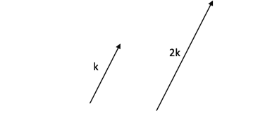
When working with vectors we can also use something called a scalar. A scalar is a number that a vector can be multiplied by in order to change the length of the vector. It is important to remember that the direction of the vector is not changed during this – only the length.
Column vectors
We can also write a vector using the notation of column vectors. This gives the same information as writing a vector using and . We must simply write them in a column. The number at the top of a column vector tells us the spaces that we move left and right and the bottom number tells us how far up and down. So any vector written with an and can be put into a column vector:
![Rendered by QuickLaTeX.com \[ 5i + 2j = \begin{pmatrix}5\\2\end{pmatrix} \]](https://b3801007.smushcdn.com/3801007/wp-content/ql-cache/quicklatex.com-ff56d6df8a5e80ea5825dedfd2396969_l3.png?lossy=2&strip=1&webp=1)
![Rendered by QuickLaTeX.com \[ 1i + 8j = \begin{pmatrix}1\\8\end{pmatrix} \]](https://b3801007.smushcdn.com/3801007/wp-content/ql-cache/quicklatex.com-51dd60cbc7161df30d45bba65dffae8f_l3.png?lossy=2&strip=1&webp=1)
This is rather easy to understand: we just move the first value for onto the top of the column vector and the second value for onto the bottom.
Example
Write the following lines as unit vectors (with and ) and as a column vector also.
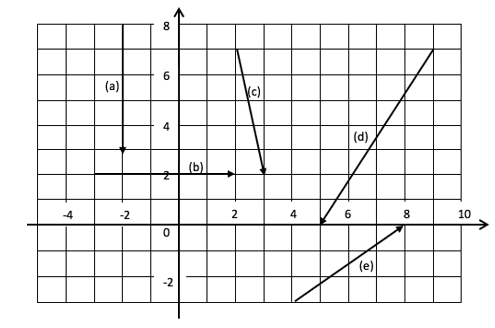
1. Remember that where the vector starts and finishes is irrelevant, we just need the size of the vector line itself. So for the first we have a line that goes straight down so the i component must be 0 and the j component is -5 squares. This gives -5j which as a column vector is:
![Rendered by QuickLaTeX.com \[ \begin{pmatrix}0\\-5\end{pmatrix} \]](https://b3801007.smushcdn.com/3801007/wp-content/ql-cache/quicklatex.com-636a47316d33b98e9dc0b2e177592fa8_l3.png?lossy=2&strip=1&webp=1)
2. Here we have an i component of 5 and a zero j component so we can write this as 5i or as the column vector
![Rendered by QuickLaTeX.com \[ \begin{pmatrix}5\\0\end{pmatrix} \]](https://b3801007.smushcdn.com/3801007/wp-content/ql-cache/quicklatex.com-dee5ea81f70b5ffd0bd70bcd1216ceeb_l3.png?lossy=2&strip=1&webp=1)
3. Here the vector has a horizontal length of 1 and a vertical length of -5. Therefore, we get i-5j and
![Rendered by QuickLaTeX.com \[ \begin{pmatrix}1\\-5\end{pmatrix} \]](https://b3801007.smushcdn.com/3801007/wp-content/ql-cache/quicklatex.com-bfac4cddf4e62e4633528e953b196fbc_l3.png?lossy=2&strip=1&webp=1)
4. Here both of the moves are negative, we have -4 in the x direction and -7 in the y. This gives a vector of -4i-7j and a column vector of
![Rendered by QuickLaTeX.com \[ \begin{pmatrix}-4\\-7\end{pmatrix} \]](https://b3801007.smushcdn.com/3801007/wp-content/ql-cache/quicklatex.com-d7f86342d6c24b36facce58268e57b75_l3.png?lossy=2&strip=1&webp=1)
5. Finally, we have a vector that moves right 4 squares and up 3. So we have 4i+3j and
![Rendered by QuickLaTeX.com \[ \begin{pmatrix}4\\3\end{pmatrix} \]](https://b3801007.smushcdn.com/3801007/wp-content/ql-cache/quicklatex.com-78fc196eecf9dab09315bc9aabfeeefd_l3.png?lossy=2&strip=1&webp=1)
Adding vectors
We can add different vectors simply by adding the different components of i and j for unit vectors or by adding the different values on the top and bottom of a column vector.
For example, (4i+3j)+(2i-2j) are both shown below, and by rearranging them so that they make one continuous line we can find the value of both of them together.
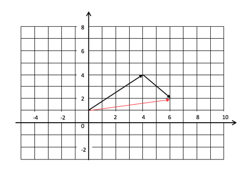
By arranging the two vectors ‘nose to tail’ (remember that the start and end points do not matter so we can move a vector and it will still be the same) we can see the effect of both vectors. These two combine to make the vector shown in red which is the same as simply adding the components of the previous two (4i+3j)+(2i-2j)=(4+2)i+(3-2)j=6i+j. So the red vector which is the combination of the two is equal to 6i+j.
The same can be done with column vectors. So:
![Rendered by QuickLaTeX.com \[ \begin{pmatrix}4\\3\end{pmatrix} + \begin{pmatrix}2\\-2\end{pmatrix} = \begin{pmatrix}4+2\\3-2\end{pmatrix} \]](https://b3801007.smushcdn.com/3801007/wp-content/ql-cache/quicklatex.com-e5118a5420b1d523bc6844f9efa5f7d0_l3.png?lossy=2&strip=1&webp=1)
which then gives the red vector as:
![Rendered by QuickLaTeX.com \[ \begin{pmatrix}6\\1\end{pmatrix} \]](https://b3801007.smushcdn.com/3801007/wp-content/ql-cache/quicklatex.com-0e20155bf7dfff416f6451109fc17894_l3.png?lossy=2&strip=1&webp=1)
Subtracting vectors
We can also subtract different vectors from each other. To do this, the vector which is being subtracted must first be multiplied by and then added (which is all that a subtraction is anyway). By multiplying the vector to be taken away by , we can draw the correct vectors out on a graph.
Example
We have the vector and wish to take away the vector . What is the resulting vector?
If we were to draw this out we would draw the vector as normal but the vector must be multiplied by before being drawn and assembled with the first vector, nose to tail. However, since we are not asked to draw the vectors we can simply do the calculation:
![Rendered by QuickLaTeX.com \[ (4i+4j) - (6i+2j) = (4-6)i + (7-2)j = -2i + 5j \]](https://b3801007.smushcdn.com/3801007/wp-content/ql-cache/quicklatex.com-5a6c9a3a7640cccada9f235b226dd99a_l3.png?lossy=2&strip=1&webp=1)
Or with column vectors we get:
![Rendered by QuickLaTeX.com \[ \begin{pmatrix}4\\7\end{pmatrix} - \begin{pmatrix}6\\2\end{pmatrix} = \begin{pmatrix}4-6\\7-2\end{pmatrix} = \begin{pmatrix}-2\\5\end{pmatrix} \]](https://b3801007.smushcdn.com/3801007/wp-content/ql-cache/quicklatex.com-61da0fa430e3bea9f4261bef75bc6881_l3.png?lossy=2&strip=1&webp=1)
Scalar multiplication
‘Scalar multiplication’ sounds complicated but it is actually very simple! A scalar is simply another word for a constant (number) which is multiplied by a vector. So if we have the vector A=3i+6j and we multiply it by the scalar 2, we get 2A=2(3i+6j)=6i+12j
It really is as simple as just multiplying each component of the vector (the i and j) by the number given! Of course, the number (or ‘scalar’) could be anything and even a fraction. But by sticking to our skills of multiplying out brackets we will easily find the answer.
Scalar multiplication with a column vector will do exactly what we expect: we multiply the top by the scalar and then multiply the bottom by the same number and leave the answer as a column vector still. So
![Rendered by QuickLaTeX.com \[ 3\begin{pmatrix}5\\-2\end{pmatrix} = \begin{pmatrix}3\times5\\3\times(-2)\end{pmatrix} = \begin{pmatrix}15\\-6\end{pmatrix} \]](https://b3801007.smushcdn.com/3801007/wp-content/ql-cache/quicklatex.com-1b2ba3250ee1338aeeca041ecb651fc6_l3.png?lossy=2&strip=1&webp=1)
Really what we are doing if we were to map the vectors is combining a given amount. So if the scalar is 3, we are finding the value of applying a vector 3 times. So for the vector 2i+j multiplied by the scalar 3 we have:
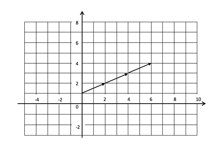
Which is clearly just the same as a vector in the same direction but 3 times as large.

