All about Graphs

Quadrants of a graph

In mathematics, it is common to represent data from situations. This is often done with the use of a graph which is a great way to show two different measurements against each other (for example, the graphs we have previously looked at that compared speed and time). A normal graph can be split into four different sections depending on the values of x and y being positive or negative. Below shows the four quadrants and what coordinates x and y must be in order to be in each.

Plotting graphs

In order to plot a graph we simply need to have values for different things. These could be anything at all and we must plot one on the horizontal (x) axis and the other on the vertical (y) axis. Each point can then be joined up or inspected to see a trend between the two things we are measuring. This will allow us to make future predictions or report on situations that have already happened.

Types of graphs

There are many different types of graphs that we can get using line equations. Which one we have will depend on the individual equation and the power of the x or y variable. From now on we will assume that the equation is separated and y is made to be the subject on the left-hand side. The types of graph that we will get will be one of the following:

x to the power of 1 – produces a straight line

x to the power of 2 – produces a u-shape or n-shape

x to the power of 3 – produces two swaps in the direction of the graph

x to the power of 1

This will always result in a line and not a curve. An example of a line like this will have an equation of  or any other combination as long as is not to any power. This looks like:

x to the power of 2

When is x squared we get a curve which has either a minimum or maximum (a specific largest point or smallest). So we get a curve which looks like either a u-shape or an n-shape.

This looks like:

x to the power of 3

When x is cubed we get a curve which changes direction twice. This can be in either direction such as the images shown below. This looks like:

All of these graphs could be slightly different in the way they look in terms of steepness and other aspects, the only thing which must stay the same is the number of times the curve changes in comparison to the power of x.

Drawing graphs by hand

When drawing a graph by hand we must follow certain steps. Firstly, we need to find some of the individual points that lie on the curve by choosing certain values of x and finding the corresponding y. When doing this you should look to find at least five points to give a good idea of where the curve will be. You should remember how many times the curve you are looking at will change in direction and make sure that you know roughly where these happen.

When we have enough points marked in we can look to join them up with a smooth, continuous curve with no gaps.

When drawing the curve you should always use a pencil and try to keep your hand to the inside of the curve.

The curve that is drawn should be very smooth and a good way to check your drawing is to pick a few random points on the curve and check that, when putting the x and y values into the curves equations, these are correct.

Linear and non-linear graphs

Graphs can be used even when we have continuous data, meaning that the numbers used can be absolutely anything and are not just whole numbers. Another advantage of a graph is that we can easily compare two things directly to one another; this then gives us a great tool to help us have an effect on the two different outcomes as we will know what sort of change (an increase or decrease) in one variable will produce on the other. For example, if we had a graph showing supply and demand of a product, a gradient could tell us how the increase in demand may make the supply go down as more people will rush to the shops to buy the product in question.

Linear or non-liner equations

When we plot a graph we can have one of two types: linear or non-linear. A linear graph basically means that when plotted we will see a straight line, hence the word linear meaning ‘line like’. Obviously, a non-linear graph will give us a curved shape when plotted.

The way to spot the difference when we are just given the equations for a line is to look if any of the variables x or y are to a power. If the variables are squared/cubed or to any other power (except 1) then the graph will be non-linear when plotted. This means that a graph with variables that do not have any powers must be linear and will form a straight line. For example:

 …. This must be linear as neither x or y are to any power of 2 or larger.

 …. This equation is non-linear as one of the powers (x) has a power of 2.

Interpolation

As we mentioned earlier, one of the things with graphs is that the numbers involved can be anything. This obviously gives us a problem when plotting graphs as we will not wish to waste time plotting every single individual point. For this reason, we use interpolation to plot a graph. This means that we simply have to mark a few points that are correct and then join this up using a smooth curve. A curve will give an estimate of the values between the ones which we have worked out exactly and this must be curved to fit the proper shape when we are dealing with a non-linear graph.

Example

Plot the following data on a graph and use a curve to connect the points.

X	1	2	3	4	5	6	7
	7	-8	-17	-20	-17	-8	7

Plotting these values on a graph we need to be very careful to ensure that we always have the x coordinate on the horizontal axis and the y coordinate on the vertical. Then we need to simply get a pencil and connect the points with a smooth flowing curve.

After plotting a graph of this sort we can use the fact that we have joined the points with a curve to make estimates for certain values that are between points which we actually worked out. This means that, without entering an x value into the original formula, we can guess at what value we would get for y. This is done by looking at the value of y in question, along the y axis, and then moving straight across to the curve and seeing what the x value is at this point. This enables us to use the graph to work out corresponding values when told either a value of x or y.

Finding a solution from a graph

Using the same example of  we can look to find a solution to the equation. This is where we are told one of the values for an unknown (usually y in this case as it is on its own) and must then work out what value the other variable must be from this. As stated above, we simply need to read along from the value given and see the corresponding value.

Example

Solve  where .

This basically means we must solve  when we substitute  in. This means that we must draw a line across where y is equal to 0 and see the corresponding x values where the curve crosses.

The line  is shown on the graph in red and this line crosses the curve in two different places: 1.4 and 6.6. This tells us that there are two solutions to this problem,  or .

This same technique will work no matter what equation we have plotted or the line that is made to get the solution. However, we may get any number of different solutions including 0, which is said to ‘have no solution’. By following the same technique of plotting the curve and then the entire line given by the solution we need, you will be able to find the answer no matter how many there may be.

Gradients

A gradient is related to a line and basically tells us how steep the line is. For this reason, a gradient is worked out as a ratio of the change in and the change in x. This ratio will tell us if the line is going up or down and how quickly. This is obviously very important as we can use this information to predict further values and see how effecting one value will change the other.

To find the increases in the two variables we must plot two points on the line in question and then create a right-angled triangle from this. Then we can use the two sides of the triangle that we created to find the difference along the axis and the difference along the y axis.

As marked on the diagram, the difference in the x axis is 7 squares and the difference in the y axis is 4. This tells us that we have a gradient of  which means that for every step of unit 1 in the x direction, we have a step of  in the y direction.

You may notice that the previous example had a gradient of less than one. This also tells us that the line must be at an angle less than 45° to the axis. This is because a line with gradient of 1 is the line  and has an angle of 45°. Therefore, any line that has a gradient of between 0 and 1 must be at a smaller angle and any that have a gradient more than one will be at an angle more than 45°.

Negative gradients

If we ever have an increase in x which results in a decrease in the value then we will get a negative gradient. This will be shown as a line which slopes down instead of up but is calculated in exactly the same way as we previously discussed. Basically, a positive gradient will give a line that looks to be going ‘uphill’ and a negative will give one that appears to be going ‘downhill’. To work out negative gradients we do the exact same as for positive by using the formula:

However, the y component will actually be decreasing and will therefore be a negative, which will give us a negative result for the gradient.

Equation of a line

When we are told the gradient of the line we can instantly tell how steep it will be, however, what we cannot do is plot the line as we do not know whereabouts it should go. Therefore, to plot a line on graph paper we must also have something called the y intercept.

The y intercept is the value that is when the line crosses the axis. With this value of y we will know that the line must pass through the point (0,y). For example, if the y intercept is 5 then the line must pass through the point (0,5) and if we know the gradient of this line we could go ahead and plot it on a graph. To show the gradient and y intercept we must make use of the line equation:

This equation has two unknowns that we have not come across before: m and c. These are the values of the gradient (m) and the intercept (c) for any particular line. With these two pieces of information we will be able to draw the line in question by putting the values of m and c into the equation and then plotting certain points for x equals 1, 2, 3 etc.

The table below shows an example of a line equation and the gradient and intercept that are associated with each.

Line equation	Gradient	Intercept
	3	9
		0
	7	-3
	-5	10
	2	6

The final equation in the set is divided by 2 since we must have just a single value of y in the equation of a line.

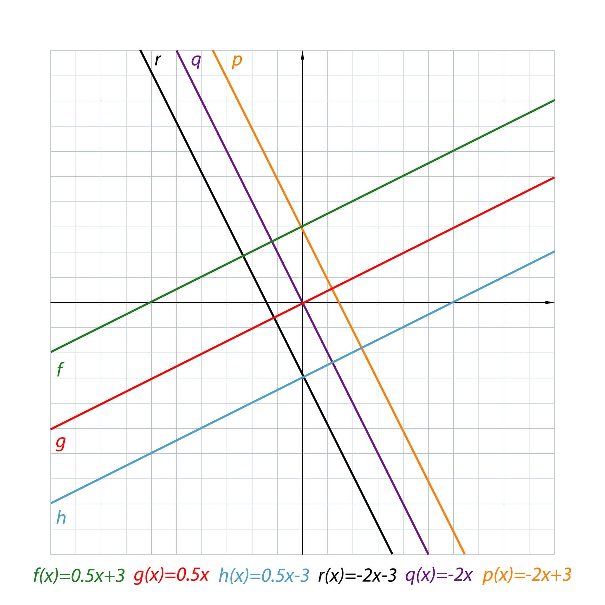
To show the effect of a different y intercept we can plot many different lines with different values for c. Then we can see the effect that this will have and why it is important to know the intercept so we can draw a line. Below are the straight lines:

All three of these lines have the same gradient and are therefore parallel, they simply move up or down according to the y intercept of each particular equation. If you look at the point where each line crosses the y  axis, these are the same as the intercept that we have from the equations given.

Finding the equation from a drawn group

If we have already been given an image of the line that we are looking at we can work out the equation for it. To do this we must work out the values of the gradient and y intercept (m and c).

Finding the gradient has already been discussed earlier: we must pick any two points on the line and then divide the difference in y by the difference in x. Then we can find the y intercept by simply seeing where the line crosses the y axis. This then lets us write an equation for the line of the form .

The lines drawn on above in red are to show the difference in the x value to the y value. The red dot is the part where the line crosses the y axis and is therefore the  y intercept. From these we can see that the gradient is 4/2 or 2 and that the y intercept is also 2. Putting these into the equation for a line we get:

This same method can be used for any line.